BCsc vignette
Raffaele A Calogero
10/01/2021
BCscvignette.RmdSection 1: Introduction
Section 1.2.1: scRNAseq QC
Section 1.3: Bray Curtis community ecology metric.
Bray Curtis metric [Bray and Curtis 1957] is a statistic used to quantify the compositional dissimilarity between two different sites, based on counts at each site. As defined by Bray and Curtis, the index of dissimilarity is:
## Warning: package 'knitr' was built under R version 3.6.2
Bray Curtis formula.
Where Cij is the sum of the lesser values for only those species in common between both sites. Si and Sj are the total number of specimens counted at both sites. The index can be simplified to 1-2C/2 = 1-C when the abundances at each site are expressed as proportions, though the two forms of the equation only produce matching results when the total number of specimens counted at both sites are the same.
The Bray-Curtis dissimilarity is always a number between 0 and 1. If 0, the two sites share all the same species; if 1, they don’t share any species.
To calculate the Bray-Curtis dissimilarity between two sites it is assumed that both sites are the same size, either in area or volume (as is relevant to species counts). This is because the equation does not include any notion of space; it works only with the counts themselves. If the two sites are not the same size, it is necessary to adjust counts before doing the Bray-Curtis calculation.
BC is fequently used in microbiome characterization to represent the dissimilarity between pairs of samples [Larsen and Dai 2015].
Example of the use of BC [Glen in www.statisticshowto.com] Lets, consider two aquariums;
- Tank one: 6 goldfish, 7 guppies and 4 rainbow fish,
- Tank two: 10 goldfish and 6 rainbow fish.
To calculate Bray-Curtis, let’s first calculate Cij (the sum of only the lesser counts for each species found in both sites). Goldfish are found on both sites; the lesser count is 6. Guppies are only on one site, so they can’t be added in here. Rainbow fish, though, are on both, and the lesser count is 4. So Cij = 6 + 4 = 10.
Si ( total number of specimens counted on site i) = 6 + 7 + 4 = 17, and Sj (total number of specimens counted on site j) = 10 + 6 = 16.
So our BCij = 1 – (2 * 10) / (17 + 16), or 0.39.
Section 1.4: Aim of the thesis.
scRNAseq is a very powerful technology, which however has still some critical points due to the high noise of the technology. A very important point, within the concept of reproducibility, is the ability to associate common clusters in independent experiments, e.g. biological replicates of the same experiment or scRNAseq from different patients with the same disease. In this thesis, I will evaluate the possibility to use Bray Curtis community ecology metric to identify common clusters in independent experiments.
Section 2: Methods
All the methods and analyses described in this thesis were generated using R. The Bray Curtis metrics (BCsc) for single cell data analysis was implemented within rCASC suite. All software for BCsc metrics was implemented in a docker container deposited at repbioinfo repository at docker hub. All calculated data are available as figshare project.
Section 2.1: Datasets
Section 2.1.1: SetA, SetB and setC
SetA, B and C were prepared to validate rCASC [Alessandri et al. 2019]. These datasets were generated combining different cell types from Zheng paper [Zheng et al. 2017]:
- setA 100 cells randomly selected for each cell type:
- B-cells, (M) Monocytes (100K reads/cell), (S) Hematopoietic stem cells, (NK) Natural Killer cells, (N) Naive T-cells
- setB 100 cells randomly selected for each cell type:
- B-cells, (M) Monocytes (100K reads/cell), (T) T-helper cells, (NK) Natural Killer cells, (N) Naive T-cells
- setC 100 cells randomly selected for each cell type:
- Monocytes, (T) T-helper cells, (NK) Natural Killer, (S) Hematopoietic stem cells
Section 2.1.2: Contaminated set: setAc30
We constructed a contaminated dataset in which a fraction of genes from setA were substituted with a random set of counts, 30%, from setC, i.e.setAc30. In figure , it shown the co-clustering of setA and setAc30.
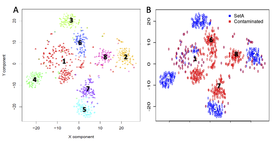
Co-clustering of setA and setAc30. A) clusters generated by seurat. B) setA and setAc30 cells
Section 2.1.3: Set1 and set2
Datasets 1 and 2 were derived from two PBMC datasets available at 10XGenomics repository. Set1 was generated usingNextGEM chemistry as instead set2 with version 3.0 chemistry.
Both datasets included antibodies labeling. Starting from these datasets we constructed set1 and 2, using the following cells:
- CD14+CD16- (Monocytes, M), CD56+CD34- (Natural Killer, NK), CD4+CD25+CD127- (T regulatory, TR), CD4+CD45RO+ccr7+ (T memory, TM), CD19+CD20+ (B cell, B), cd8+cd45ra+ccr7+ (naive T, N)
100 cells were collected for each cell type in the two experiments. Cells were cleaned up removing all cell with more than 10% mitochondrial genes. Duplicated cells, i.e. those cells showing inconsistent surface makers were removed. Genes were filtered selecting the top 10000 most variant genes and from them the top 5000 most expressed.
set1: 94 M, 95 NK, 85 TR, 62 TM, 96 B, 86 N
set2: 97 M, 94 NK, 84 TR, 82 TM, 92 B, 95 N
Section 3: Results
Section 3.1: Evaluating BC metrics efficacy, as cluster association tool, by mean of cluster-specific GO terms.
In this section we describe the results referring to the hypothesis that cell sub-popuplations (clusters) can be assimilated to microbial communities and cluster-specific enriched GO terms are assimilated to microbial philum. Thus, Bray Curtis (BC) can be used to measure the dissimilarity between any cluster of an experiment and any cluster of the other experiment, to identify those clusters that are in common between different experiments. These data try to define the limits of BC in samples that are relatively similar to each other.
SetA (500 cells), B (450 cells) and C (440 cells) were independently filtered to keep the 10k most variant genes. The retained genes were further filtered to keep the 5k most expressed genes. This passage was done to remove from each dataset the genes that, being little expressed or uniformly expressed, are going to have limited impact in clusters definition.
Each dataset was clustered with the clustering tool, within those available in rCASC [Alessandri et al. 2019], providing the best CSS score, which is a measure of cluster stability [Alessandri et al. 2019], Fig. .
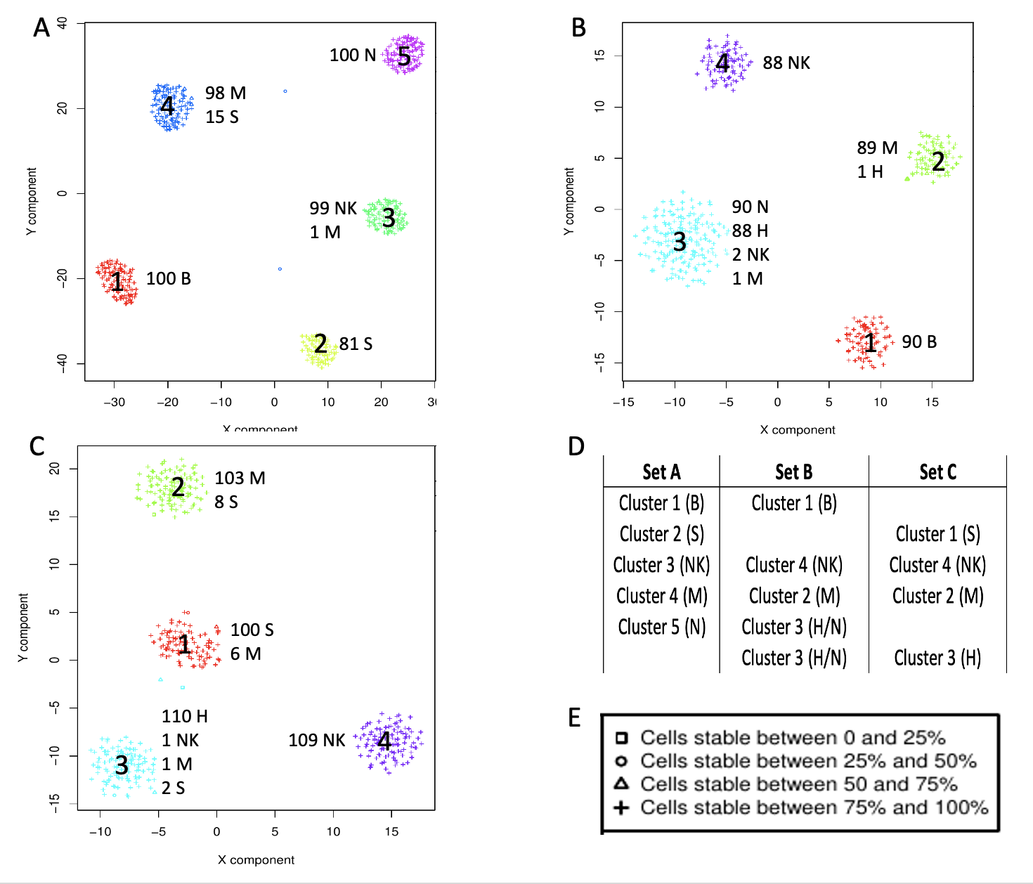
rCASC clustering. A) SetA clustered by Griph. B) SetB clustered by SHARP. C) SetC clustered by SHARP. D) Association between clusters in the three datasets. E) Legend for the CSS
As shown in Fig. , the three datasets were characterized by high CSS. Only in set B one cluster, 3, is composed mainly by two cell types, N and H cells, Fig. B. This is due to the limited sensitivity of the version 1 chemistry that was used for the generation of the data used in this experiment [Zheng et al. 2017].
Section 3.1.1: Evaluating BC metrics efficacy, as cluster association tool, by mean of cluster-specific GO terms on setA and setA depleted of a 5, 10 and 15% randomly selected genes.
To estimate the ability of BC metric to associate the same cell sub-types in different experiments, we compared setA with respect of setA in which a random subset of 5%, 10% and 15% of cells were removed. SetA and the depleted datasets were independently clustered using SIMLR, imposing 5 clusters. Each cluster was then described as a population of GO enriched terms, derived from the cluster-specific genes detected by COMET. We present only the results obtained using the biological process GO class, because the molecular function GO class was very ineffective in generating the correct association of the clusters.
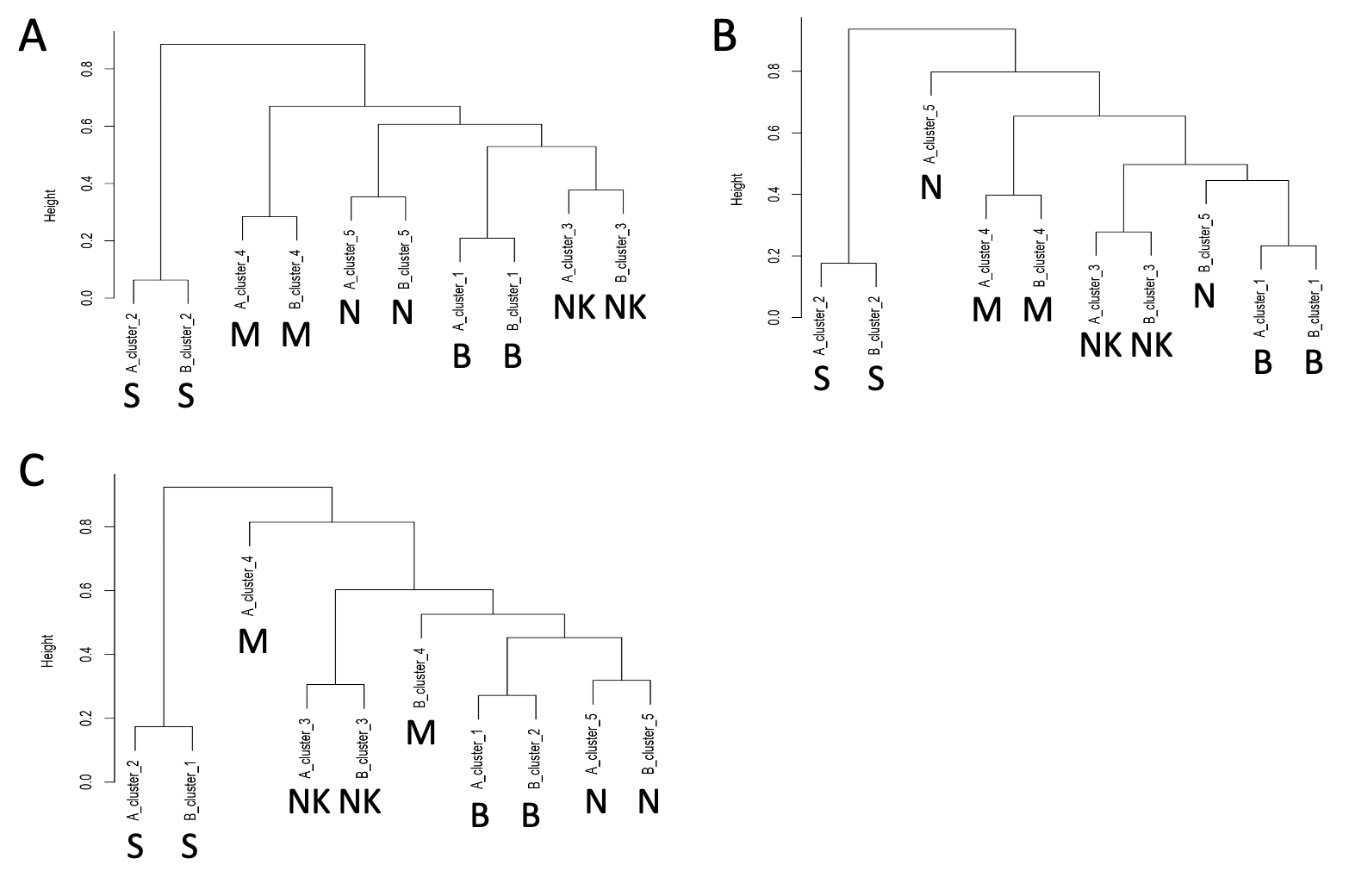
SIMLR clustering with k=5. A) Hierarchical clustering of the BC distance between setA and setA depleted of 5% cells. B) Hierarchical clustering of the BC distance between setA and setA depleted of 10% cells. C) Hierarchical clustering of the BC distance between setA and setA depleted of 15% cells
In Fig. , hierarchical clustering of BC distance suggests that BC is capturing similarity between the analyzed cell sets, even if part of the information is lost. This is however, not sufficient to say that BC is a good metric to detect common sub-populations of cells in different experiments.
We extended this analysis generating, starting from setA, two random sets each one with 5% or 10% or 20%, 30, 40% and 50% random removal of genes. Each pair of data with the same percentage of genes removal was filtered to select the top 10k most varying genes. Each dataset was clustered with Griph and COMET was applied to identify cluster-specific genes. GO enrichment was performed and BC was used to associate clusters within the two datasets. This analysis was repeated 100 times. A threshold for BC, < 0.2, was used to define if two clusters are associated to each other.
BC based association between clusters, comparing two set of samples where 50% of the genes where randomly removed. The assignement of identify between two clusters was done using the lowest BC score below the threshold that was set to 0.2, over 100 permutations. A) SetA with two different set of genes removal. B) setA1 and setA2 with two different set of genes removal.
This experiment demonstrated that, even with a large removal of genes, BC was able to associate correctly the clusters, i.e. in the worst case 72 times over 100 permutation, Fig. A.
The experiment was repeated using the same approach, but on two independent set of cells with the same cell types of setA. In Fig. B only 50% random removal of genes was described since it is the one that most strongly affect the detection efficacy of BC.
Section 3.1.2: Testing BC metrics efficacy, as cluster association tool, by mean of cluster-specific GO terms searching common clusters between setA and setB/C.
We extended the above describe analysis comparing setA, setB and setC, which are coming from the same bulk experiment but are made of different cells and with a different composition of cell types, for their composition see Methods section. Each dataset was analyzed with COMET to identify the subset of genes most characteristic of each cluster. Each of these set of genes was used to search for enriched GO terms using topGO Bioconductor package. Subsequently, we investigated if BC could provide an effecting tool to detect corresponding clusters in different experiment, Fig. .
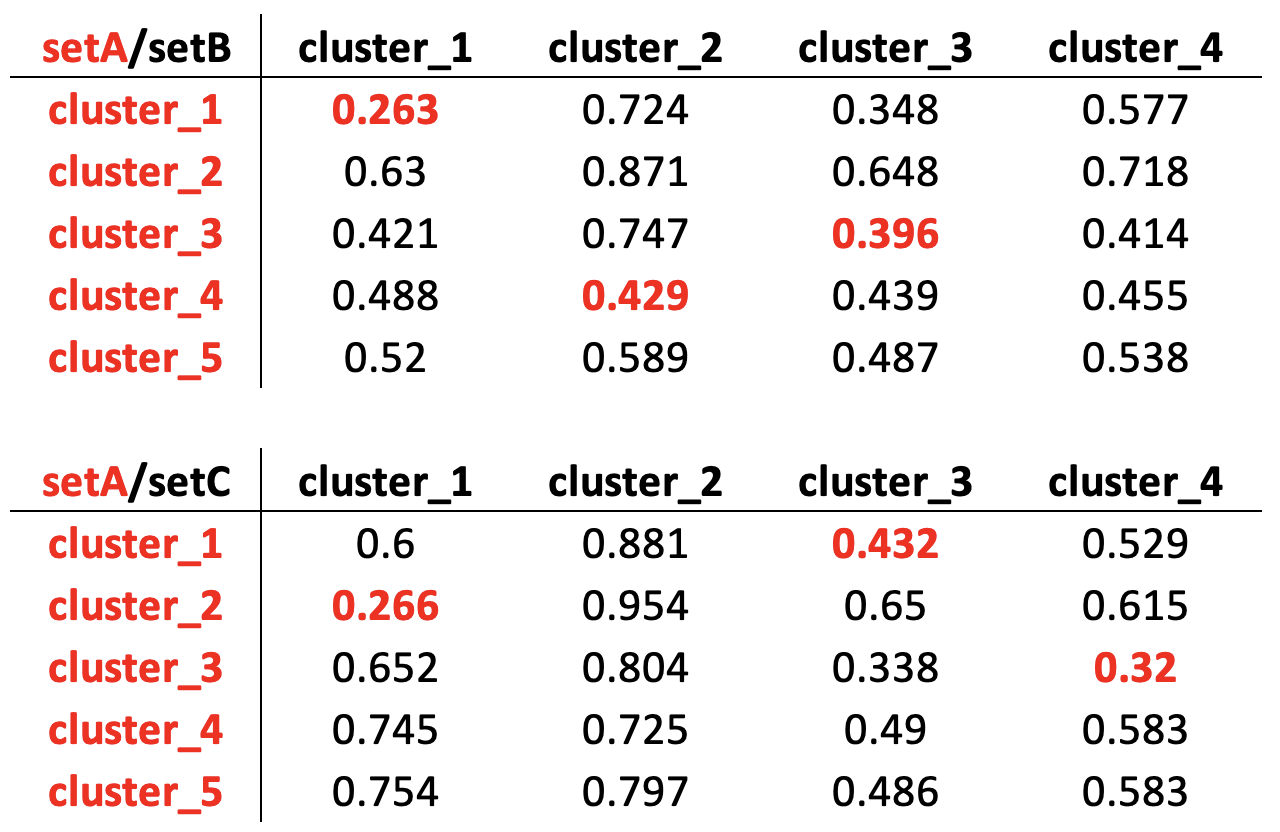
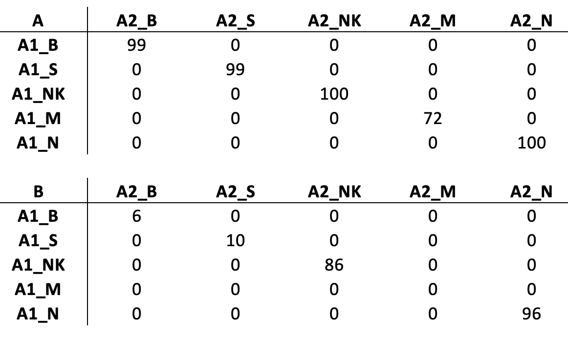
Measuring cluster to cluster dissimilarity using Bray Curtis metric applied on cluster-specific enriched GO terms.
Looking at the lower values of BC between the clusters in setA and B, Fig. setA versus setB red values, we correctly assigned the B cells and M cells clusters but we failed in correctly assign the NK cluster in setB. In the case of setA versus setC, S cells and NK cells clusters were correctly associated. Instead setA B cells, which are not included in setC, were incorrectly associated to H cells in setC.
The results obtained trying to identify cluster to cluster association between different datasets highlight the present of two critical points associated to this approach: i. the idea of detecting clusters relationship starting from the minimal BC value provides only a partial correct association between clusters; ii. in case a cluster is not shared between different samples the BC scoring approach we have used does not support this issue. Furthermore, we have also observed that GO enrichment on cluster-specific genes sometimes produces very short list of GO terms, reducing the ability of BC in measuring correctly the dissimilarity between samples.
Section 3.2: Testing BC metrics efficacy, as cluster association tool, by mean of cluster-specific genes.
In the previous experiments, we observed that GO terms associated to cluster-specific genes, in some cases were very few, thus limiting the strength of BC score in cluster association. Then, we decided to directly use BC score on cluster-specific genes.
Section 3.2.1: Creation of the contaminated dataset setAc30
We investigated the efficacy of BC score on cluster-specific genes comparing setA with respect to a setA contaminated by randomly selected genes from setC. Specifically, we have transformed setA contaminating it with 30% of the setC counts, randomly selected.
In brief, descrivere come hai fatto la contaminazione
**parte ancora da completare
Section 3.3: Analysis of pbmc_NextGEM and pbmc_v3_chemistry
pbmc_NextGEM dataset is the dataset made of 5k Peripheral blood mononuclear cells (PBMCs) from a healthy donor with cell surface proteins (Next GEM) available at 10XGenomics repository.
pbmc_v3_chemistry dataset is the dataset made of 5k Peripheral blood mononuclear cells (PBMCs) from a healthy donor with cell surface proteins (v3 chemistry) available at 10XGenomics repository.
Both datasets were analysed in the following way:
Low quality cells, i.e. those containing less that 100 genes were removed. All cells with a ribosomal gene percentage between 10 and 70% and a mitochondrial percentage between 1 and 20% were also retained.
10K most variable genes were selected and out of them 5K most expressed genes were selected.
Seurat [Stuart et al. 2019] was used to cluster the data using the first 5 PCA components.
Cluster specific gene prioritization was done with COMET software [Delaney et al. 2019].
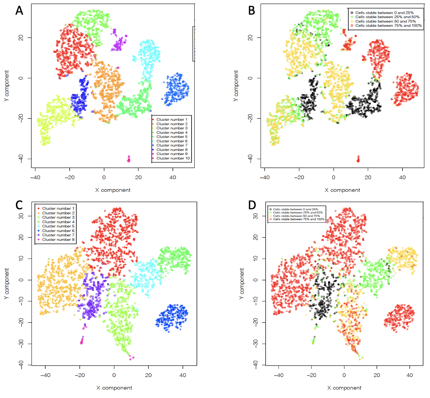
rCASC clustering. A) pbmc NextGEM 10 clusters. B) pbmc NextGEM CSS. C) pbmc v3 chemistry 8 clusters. D) pbmc v3 chemistry CSS
We detected a total of 10 clusters for pbmc_NextGEM, 7 of them with high CSS score, Fig. AB, and 8 clusters for pbmc_v3_chemistry, 6 of them with high CSS, Fig. CD.
These datasets incorporate a panel of 31 TotalSeq antibodies (BioLegend) that were used to assign the cell types for set1 and set2: CD3, CD4, CD8a, CD11b, CD14, CD15, CD16, CD19, CD20, CD25, CD27, CD28, CD34, CD45RA, CD45RO, CD56, CD62L, CD69, CD80, CD86, CD127, CD137, CD197, CD274, CD278, CD335, PD-1, HLA-DR, TIGIT, IgG1, IgG2a, IgG2b.
Analysis of set1 and set2
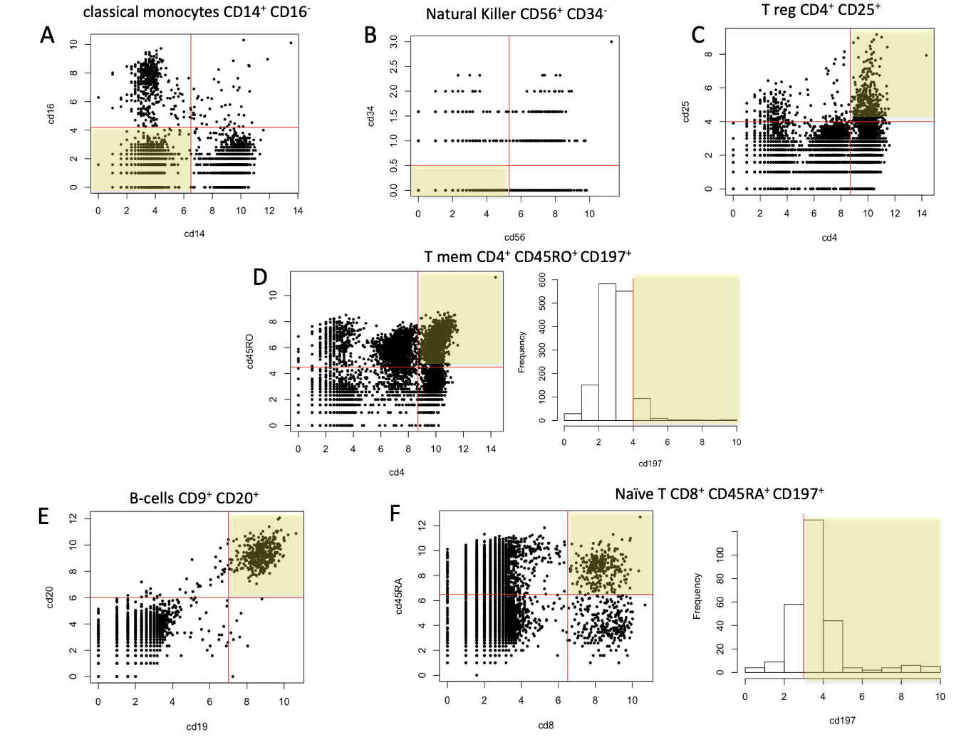
Cell type assignment. A) classical monocytes. B) Natural Killer cells. C) pbmc_v3_chemistry 8 clusters. C) T-regulatory cells. D) T memory cells. E) B-cells. F) naive T cells
In Fig. , are summarised the filters applied to the different combinations of Abs to obtain the subsets of cells we were interested in set1 and 2.
After sub-population selection, from each population the first 100 cells were selected or in case of fewer cell, all cell were selected. Only cell characterized by a mitochondrial genes percentage between 1 and 10 were kept.
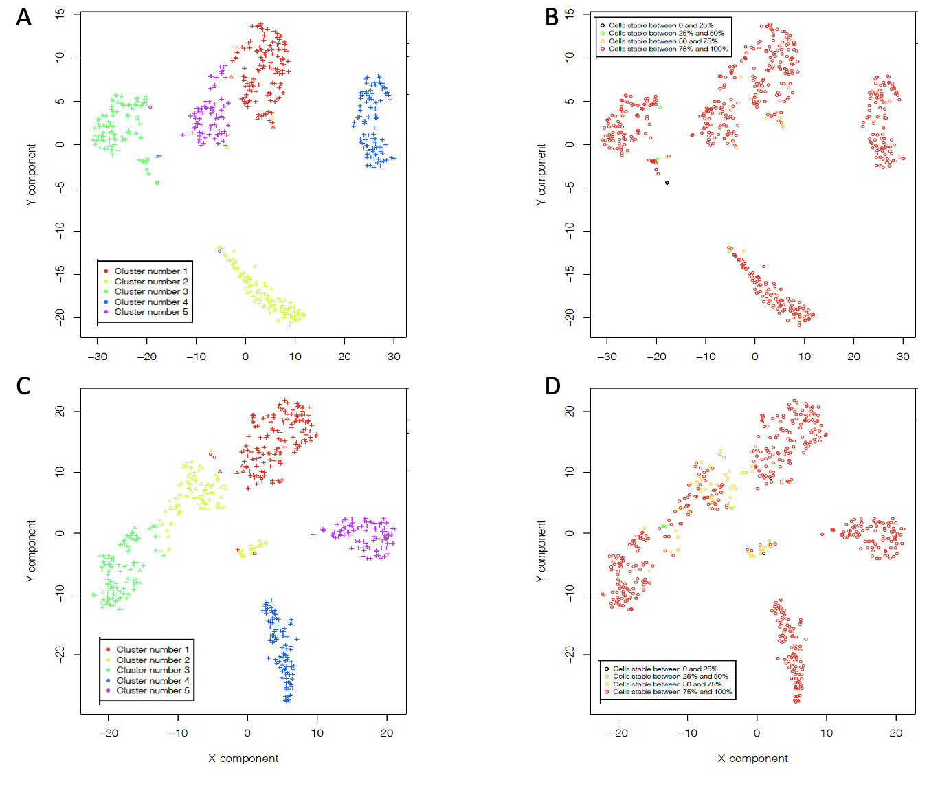
rCASC clustering. A) set1 clusters. B) set1 CSS. C) set 2 clusters. D) set2 CSS
Inconsistent cells, i.e. cells associated at more that one cell type were removed. 10K most variable genes were selected and out of them 5K most expressed genes were selected. The remain cells were clustered as described for pbmc_NextGEM and pbmc_v3_chemistry. In both cases we obtained 5 clusters, all with very good stability, Fig. .
The content of all clusters is quite homogeneous but those containing T derived cells. naive T cell clusters are contaminated by Tmem (TM) and Treg (TR) cells. The cluster of TR has some contamination by TM, Fig. .
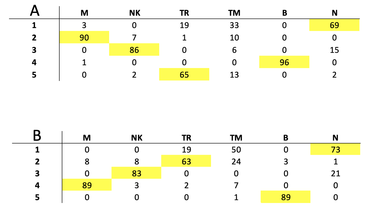
Clusters cell type content. A) set1. B) set2.