Section 1: Brief introduction on Sparsely-Connected-Autoencoder (SCA) analysis

The scRNAseq analysis tools, which are part of the rCASC package [Alessandri et al 2019], are implemented in docker containers to simplify the installation procedure of the overall workflow and to guarantee functional and computational reproducibility [Kulkarni et al. 2018]. Figure below shows the overall organization of rCASC.

## Warning: package 'knitr' was built under R version 3.6.2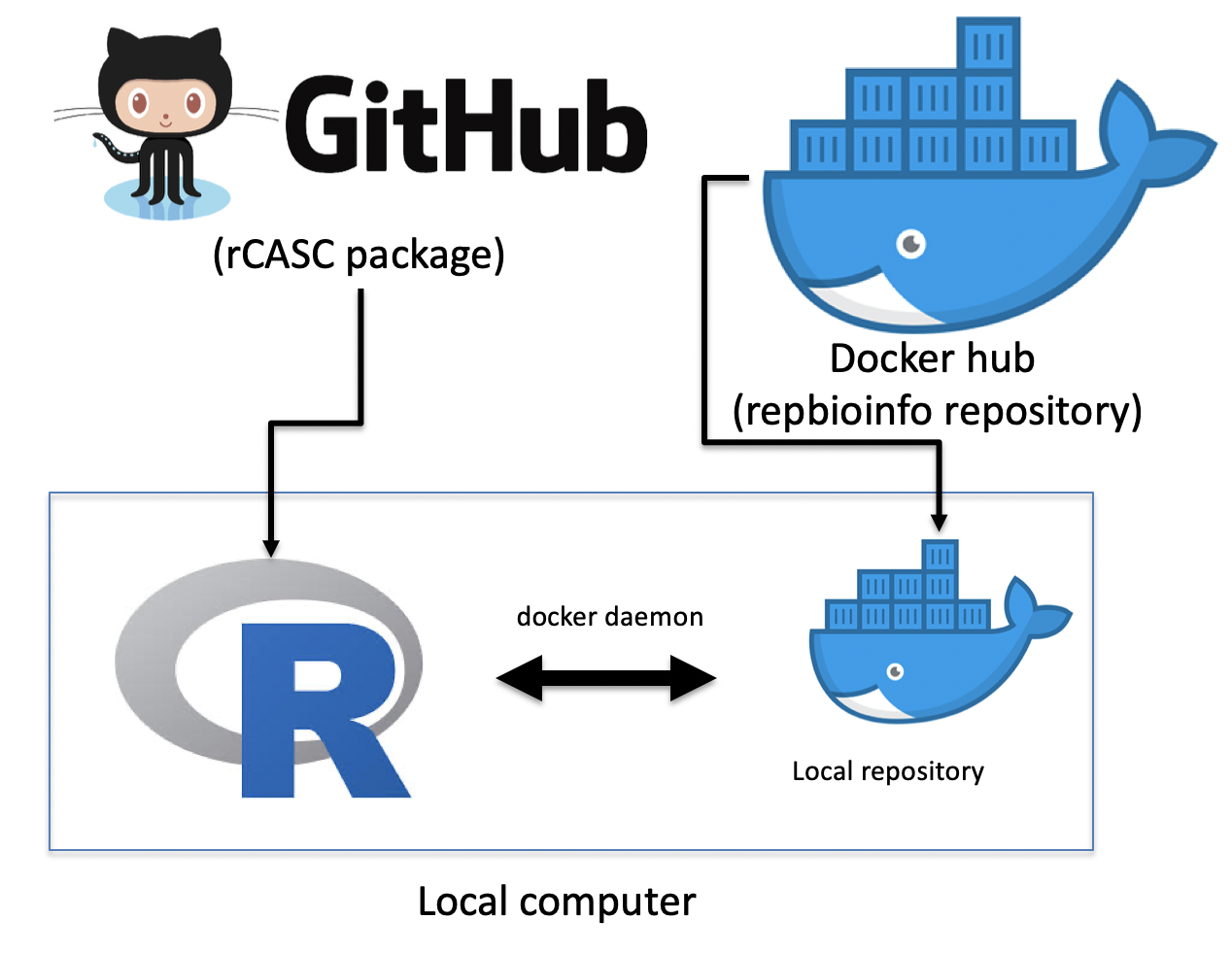

Figure rCASC organization. rCASC is available as R package in github repository. rCASC can be installed locally using install_github function from devtools R library. A local installation of the docker images required for the analysis can be done with downloadContainers function of rCASC package. A local installation of rCASC acts as workflow manage, which interacts with the local docker repository via a specific daemon, to execute scRNAseq data analyses

The SCA workflow is shown in the figure below, which describes the basic steps required to extract hidden functional features, i.e. TFs, miRNAs, Kinases, from a scRNAseq experiment using Sparsely-Connected-Autoencoder. To execute a SCA analysis it is required a scRNAseq count matrix. Subpopulation organization is then discovered using any of the clustering tools implemented in rCASC a), and the quality of the subpopulation organization is evaluated using Cell Stability Score metric b), for more info on CSS please see [Alessandri et al 2019 supplementary data. The clusters’data matrix, which is the count matrix including subpopulation organization, is normalized c). Normalized data are used to train a Sparsely-Connected-Autoencoder d). The hidden layer matrix is saved over multiple runs of the Sparsely-Connected-Autoencoder (hidden layer matrix is made of 0/1 for each hidden node, where 1 indicates that the node was used and 0 that the node was not used). The ability of each hidden layer matrix to reconstruct, at least partially, the expected subpopulation organization is evaluated by clustering e) and the quality of the reconstruction is evaluated using two metrics: Quality Control of Clusters and Quality Control of Models f), more information on these two metrics will be given later in this vignette. The hidden layer frequency matrix provides information of the usage of the hidden nodes (TFs, miRNAs, Kinases) over multiple runs of the Sparsely-Connected-Autoencoder. COMET tool [Delaney et al. 2019] is then used to grab the most important molecular features, i.e. TFs, miRNAs, Kinases, associated to each SCA reconstructed cluster.

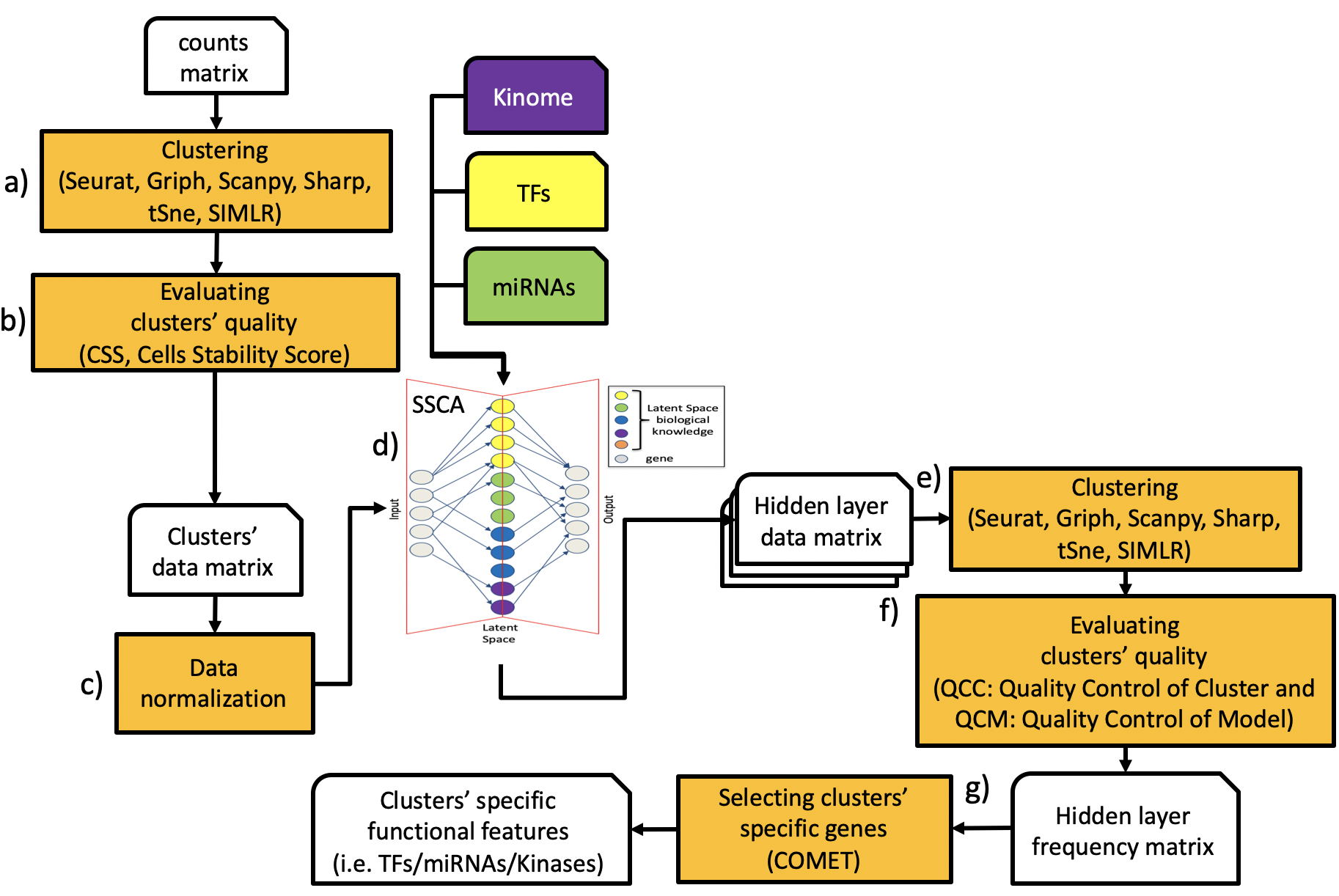
Figure SCA workflow

Section 2: Dataset used in this vignette to demonstrate the use of SCA analysis.

A data set, setA [Alessandri et al. 2019], based on FACS purified cell types [Zheng et al. 2017] was used to investigate the SCA behaviour.

setA: 100 cells randomly selected for each cell type

B-cells (B, 25K reads/cell),
Monocytes (M, 100K reads/cell),
Stem cells (HSC, 24.7K reads/cell),
Natural Killer cells (NK, 29K reads/cell),
Naive T-cells (N, 19K reads/cell)

SetA was previously used to estimate the strength of CSS metric [Alessandri et al. 2019]. We clustered setA using all the clustering tools actually implemented in rCASC: tSne+k-mean [Pezzotti et al. 2017], SIMLR [Wang et al. 2017], griph [Serra et al. 2019], Seurat [Butler et al. 2018], scanpy [Wolf et al. 2018] and SHARP [Wan et al. 2020]. All tools but tSne+k-mean and scanpy provided very good and similar partition of the different cell types (see Figure below).

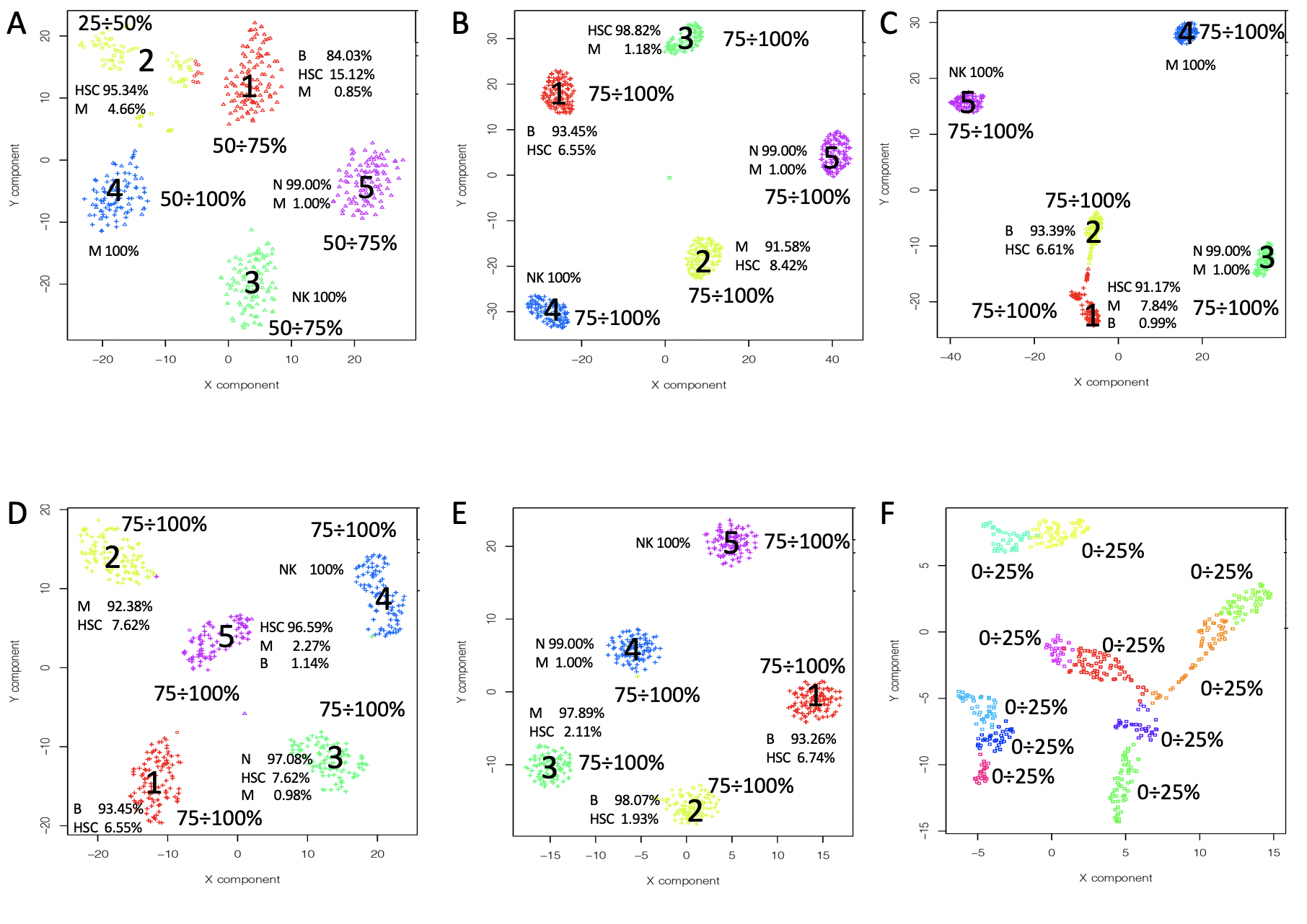
Figure SetA clustering. These results are based on the analysis of a log10 transformed count matrix.

Section 3: Manually curated cancer-immune-signature

SCA analysis based on a manually curated cancer-immune-signature (IS, Figure below) was also used on setA reference clusters, see main manuscript. This SCA analysis shows, for cluster 4 (Natural Killer cells) and cluster 5 (Naïve T-cells), QCM/QCC values greater than 0.5 for the majority of the cells (Figure below).

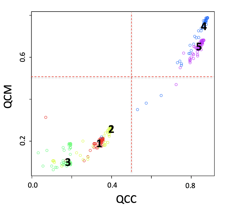
Figure SCA analysis using a manually curated cancer-immune-signature (IS). Input counts table for SCA is setA, log10 transformed. 160 permutations were run and latent space clustering was done with SIMLR.

Section 4: variational SCA (vSCA)

VAEs have one fundamentally unique property that separates them from other autoencoders: their latent spaces are, by design, continuous, allowing easy random sampling and interpolation. We tested vSCA based on TF-targets using setA. Looking at the results at the level of QCC and QCM, vSCA does not provide any advantage with respect to a normal SCA, see Figure below.

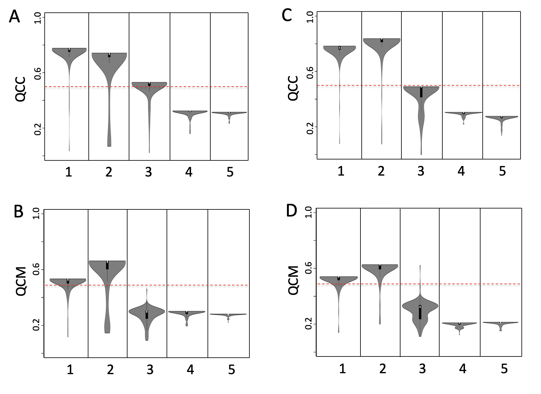
Figure vSCA based on TFs targets. A) QCC TFs based SCA, B) QCM TFs based SCA, C) QCC TFs based vSCA, D) QCM TFs based vSCA . Input counts table for SCA is log10 transformed, analysis was performed using 160 permutations and latent space clustering was done with SIMLR.

Section 5: How to run a SCA analysis.

This section provides an example of a SCA analysis, number of permutations is kept very small to reduce computing time.

The overall run described in this vignette is available in the folder vignettes/setA

IMPORTANT: Please note that the results generated in this section are meaningless. They are only used to demonstrate the how SCA functions work. In a real experiment at least 120 permutations MUST be execute in each chunk of code, where permutations are indicated.

Computing time, in each chunk, refers the time required to execute the task on a MacBook Pro (3.5 GHz Dual-Core Intel Core i7, 16 Gb RAM).

Section 5.1: autoencoder function

The input data for the autoencoder function are generated using the following script. As clustering tool we have used Griph [Serra et al. 2019], Seurat [Butler et al. 2018].

start_time <- Sys.time()

library(rCASC)
home <- getwd()
# cat("\n",home,"\n")
dir.create(paste(home, "setA", sep="/"))
dir.create(paste(home, "scratch", sep="/"))

## Warning in dir.create(paste(home, "scratch", sep = "/")): '/Users/
## raffaelecalogero/Dropbox/data/partially-connected-autoencoders/paper/
## npj_Systems_Biology_and_Applications/rebuttal/SCAtutorial/vignettes/scratch'
## already exists

file.copy(from=paste(path.package("rCASC"),"examples/setA.csv.zip", sep="/"), to=paste(home, "setA", sep="/"), overwrite = T)

## [1] TRUE

unzip(paste(home, "setA/setA.csv.zip", sep="/"), exdir=paste(home, "setA", sep="/"))
file.remove(paste(home, "setA/setA.csv.zip", sep="/"))

## [1] TRUE

system(paste("rm -fR ", home,"/setA/__MACOSX", sep=""))

griphBootstrap(group="docker",scratch.folder=paste(home, "scratch", sep="/"), file=paste(home, "setA/setA.csv", sep="/"),  nPerm=8, permAtTime=8, percent=10, separator=",",logTen=0, seed=111)

## 
##  In your system the following version of Docker is installed:
## Docker version 19.03.12, build 48a66213fe
## creating a folder in scratch folder
## 
## Docker ID is:
##  922444fa6fd7 
## ................
## 
## 
## Docker exit status: 0 
## Copying Result Folder
## 
## Removing the temporary file ....
## 
##  In your system the following version of Docker is installed:
## Docker version 19.03.12, build 48a66213fe
## creating a folder in scratch folder
## 
## Docker ID is:
##  a2238aa22e9a 
## ...
## 
## 
## Docker exit status: 0 
## Copying Result Folder
## 
## Removing the temporary file ....

end_time <- Sys.time()
cat("\n Computing time: ",end_time - start_time, " mins\n")

## 
##  Computing time:  2.909978  mins

The autoencoder function feeds the SCA using the data derived by the script shown above. The chunk below show a single permutation run, which is used to estimate the nEpochs max value. Figure learning rate shows an example of the learning curve. In this example the maximum level of learning is obtained with 250 epochs. Thus, the analysis with multiple permutations can be done setting epoch slightly greater than 250, e.g. 300. Learning pictures are saved in SCAtutorial/vignettes/setA/Results/setATF/5/

start_time <- Sys.time()

library(rCASC)
home <- getwd()
# cat("\n",home,"\n")
autoencoder(group=c("docker"),
            scratch=paste(home, "scratch", sep="/"),
            file=paste(home, "setA/setA.csv", sep="/"),
            separator=",", nCluster=5, bias="TF", permutation=1,
            nEpochs=2000, patiencePercentage=5,
            cl=paste(home, "setA/Results/setA/5/setA_clustering.output.csv", sep="/"),
            seed=1111, projectName="setATF", bN="NULL")

## 
##  In your system the following version of Docker is installed:
## Docker version 19.03.12, build 48a66213fe
## creating a folder in scratch folder
## [1] "setA_clustering.output.csv"
## 
## Docker ID is:
##  58653b2b66a7 
## .........
## 
## 
## Docker exit status: 0 
## Copying Result Folder
## 
## Removing the temporary file ....

end_time <- Sys.time()
cat("\n Computing time: ",end_time - start_time, " mins\n")

## 
##  Computing time:  1.364335  mins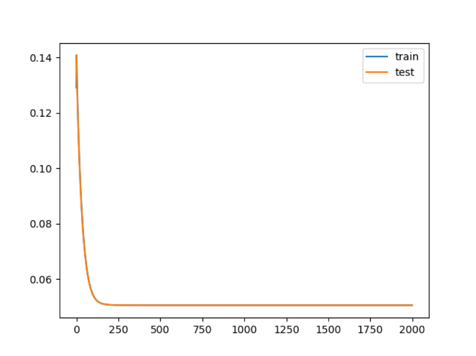

Figure learning rate.

Section 5.1.1: autoencoder parameters (for the full list of parameters please refer to the function help):

group, usually set to docker, indicating the group of users allowed to execute docker instances.
scratch.folder, a character string indicating the path of the scratch folder. Usually scratch folder is located on a SSD disk to guarantee optimal IO.
file, a character string indicating the path of the count matrix, it includes count matrix name with extension.
bias, 6 options are available: “mirna” , “TF”, “CUSTOM”, “kinasi”,“immunoSignature”, “ALL”. This parameter refers to the rules used to generate the partially connected hidden layer. If ALL is used, mirna, TF, kinasi, immunoSignature are combined to generate a SSCA (Sparse-Sparsely-Connected-Autoencoder). If CUSTOM is selected the path to the file required to build the autoencoder structure should be assigned to the parameter bN. The hidden layer description file must have the following structure source (header is mandatory and row names must not be present, any extra column will be not taken in account):
- name of the hidden layer node, column 1
- geneTarget, i.e. genes present in the hidden node, column 2.
nEpochs, this is the parameter referring to the number of times the training vectors are used to update the hidden layers weights. At the end of this learning step the best weights for nodes are defined. Please note that the best weights are not necessarily in the last epoch. Frequently, they are located in the first 1000 epochs. Thus, a good approach is to run 2000 epochs with 1 permutation only and check the learning rate, see figure below. The optimal epochs is selected within the flat part of the learning curve. Then, the analysis is run again with the number of permutations of your choice.
permutation, this parameter refers to the number of times the neural network is calculated from scratch. The number of permutations depends on the level of consistency requested, usually 160 permutations provides robust results, but it might take some times to execute on a common laptop.
cl, this parameter refers to the full path to the _clustering.output file to be used, which was generated using rCASC clustering, see the output of the above chunk of code.
ProjectName parameter refers to the name of the folder where autoencoder outputs will be saved.

start_time <- Sys.time()

library(rCASC)
home <- getwd()
# cat("\n",home,"\n")
autoencoder(group=c("docker"),
            scratch=paste(home, "scratch", sep="/"),
            file=paste(home, "setA/setA.csv", sep="/"),
            separator=",", nCluster=5, bias="TF", permutation=8,
            nEpochs=300, patiencePercentage=5,
            cl=paste(home, "setA/Results/setA/5/setA_clustering.output.csv", sep="/"),
            seed=1111, projectName="setATF", bN="NULL")

## 
##  In your system the following version of Docker is installed:
## Docker version 19.03.12, build 48a66213fe
## creating a folder in scratch folder
## [1] "setA_clustering.output.csv"
## 
## Docker ID is:
##  f71dff9f9ea3 
## ..............
## 
## 
## Docker exit status: 0 
## Copying Result Folder
## 
## Removing the temporary file ....

end_time <- Sys.time()
cat("\n Computing time: ",end_time - start_time, " mins\n")

## 
##  Computing time:  2.205505  mins

The autoencoder function produces as output many files with the extension Ndensespace.format, in the folder Results/ProjectName/Permutation. The number of such files corresponds to the number of selected permutations. In this specific examples autoencoder outputs are in /SCAtutorial/vignettes/setA/Results/setATF/5/permutation/ folder.

Section 5.2: autoencoderClustering function

The function autoencoderClustering generates the numerical data required to understand if there is coherence between counts table derived clusters and those derived using autoencoders latent space.

start_time <- Sys.time()

home <- getwd()
# cat("\n",home,"\n")
library(rCASC)
autoencoderClustering(group="docker", scratch.folder=paste(home, "scratch", sep="/"),
                      file=paste(home, "setA/Results/setATF/setA.csv", sep="/"),
                      separator=",", nCluster=5, clusterMethod="GRIPH", seed=1111,
                      projectName="setATF", permAtTime=8)

## 
##  In your system the following version of Docker is installed:
## Docker version 19.03.12, build 48a66213fe
## creating a folder in scratch folder
## 
## Docker ID is:
##  bf11bbea4533 
## ........
## 
## 
## Docker exit status: 0 
## Copying Result Folder
## 
## Removing the temporary file ....

end_time <- Sys.time()
cat("\n Computing time: ",end_time - start_time, "\n")

## 
##  Computing time:  1.201699

Section 5.2.1: autoencoderClustering parameters (for the full list of parameters please refer to the function help):

file, (IMPORTANT NOTE) this parameter refers to the full path of the count table copied in the results output folder of the autoencoder function. See as example the above chunk of code
projectName, this parameter is the same indicated in autoencoder function.
clusterMethod, this parameter refers to any of the clustering methods available in rCASC (“GRIPH”,“SIMLR”,“SEURAT”,“SHARP”), not necessary should be the same used for the raw count table clustering, actually it is useful to test more than one clustering method to see which one provides the best convergence with the clusters initially generated using the genes counts table.
pcaDimensions, this parameter is only required when Seurat is used as clustering tool.

The autoencoderClustering output is a folder where the name is given by the combination of the projectName and the clusterMethod, e.g in the above example /Results/setATF_GRIPH. In the example above, in the folder /SCAtutorial/vignettes/setA/Results/setATF_GRIPH/5/, there is the file label.csv, where is located the cluster assignment for each cells over each permutation.

Section 5.3: autoencoderAnalysis function

The output of autoencoderClustering is used by the function autoencoderAnalysis to generate the QCC and QCM statistics. QCC is an extension of CSS, for a complete mathematical description of CSS please see [Section 5.1 Cell Stability Score: mathematical description in Alessandri et al. 2019 supplementary data] and it measures the ability of latent space to keep aggregated cells belonging to predefined clusters generated using the gene count table. The metrics has the range between 0 and 1, where 1 indicates a high coexistence of cells within the same cluster in the analysis, and 0 a total lack of coexistence of cells within the same cluster.

start_time <- Sys.time()

home <- getwd()
cat("\n",home,"\n")

## 
##  /Users/raffaelecalogero/Dropbox/data/partially-connected-autoencoders/paper/npj_Systems_Biology_and_Applications/rebuttal/SCAtutorial/vignettes

library(rCASC)
autoencoderAnalysis(group="docker", scratch.folder=paste(home, "scratch", sep="/"),
                    file=paste(home, "setA/Results/setATF_GRIPH/setA.csv", sep="/"),
                    separator=",", nCluster=5, seed=1111,
                    projectName="setATF_GRIPH", Sp=0.8)

## 
##  In your system the following version of Docker is installed:
## Docker version 19.03.12, build 48a66213fe
## creating a folder in scratch folder
## 
## Docker ID is:
##  32a26acafebe 
## ..
## 
## 
## Docker exit status: 0 
## Copying Result Folder
## 
## Removing the temporary file ....

end_time <- Sys.time()
cat("\n Computing time: ",end_time - start_time, "\n")

## 
##  Computing time:  11.8868

In the figure below, only cluster 7 can be well explained by latent space, Figure below panel B. QCM metric is also an extension of CSS and it measures the ability of the neural network to generate consistent data over the different training. In the Figure below panel C, SCA provides consistent data only for clusters 5 and 7. Informative clusters are those characterized by high QCM and QCC scores. In Figure below panel D, only cluster 7 is characterized by a robust neural network able to keep the cell aggregated using hidden layer knowledge. Dashed red line (Figure below panel D) indicates the defined threshold to consider the latent space information suitable to support cells’ clusters.

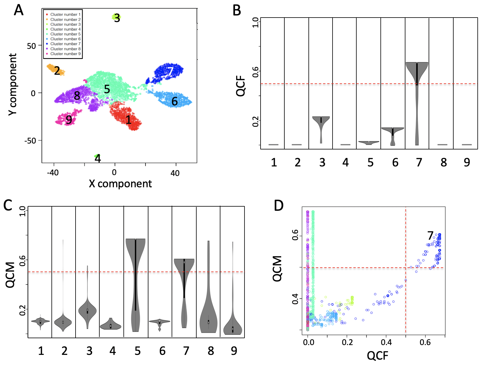
Figure QCC and QCM. Summary generated using output of autoencoderAnalysis for the Breast cancer data set in Fig. 5 main manuscript. A) Nine clusters were detected analysing breast cancer dataset with SIMLR. B) QCC violin plot. C) QCM violin plot, D) Combined view of QCM and QCC

Section 5.3.1: autoencoderAnalysis parameters (for the full list of parameters please refer to the function help):

file, (IMPORTANT NOTE) this parameter refers to the full path of the count table copied in the results output folder of the autoencoderClustering function. See as example the above chunk of code (same as for autoencoderClustering function)
projectName, this parameter is the same indicated in autoencoderClustering function.
sp, this parameter indicates the similarity threshold defined for CSS, default 0.8. Reduction below 0.7 of this threshold reduces the specificity of CSS; values equal or smaller than 0.5 are meaningless.

The outputs of autoencoderAnalysis are the pdfs:

_stabilityPlot.pdf (QCC, Figure above panel B)
_stabilityPlotUNBIAS.pdf (QCM, Figure above panel C)
_StabilitySignificativityJittered.pdf (QCM versus QCC, Figure above panel D)

The above files are saved in setA/Results/setATF/5/

Section 5.4: autoFeature function

The autoFeature creates the frequency table for COMET analysis [Delaney et al. 2019].

start_time <- Sys.time()

home <- getwd()
cat("\n",home,"\n")

## 
##  /Users/raffaelecalogero/Dropbox/data/partially-connected-autoencoders/paper/npj_Systems_Biology_and_Applications/rebuttal/SCAtutorial/vignettes

library(rCASC)
autoFeature(group="docker", scratch.folder=paste(home, "scratch", sep="/"),
            file=paste(home, "setA/Results/setATF_GRIPH/setA.csv", sep="/"),
            separator=",", nCluster=5, projectName="setATF_GRIPH")

## 
##  In your system the following version of Docker is installed:
## Docker version 19.03.12, build 48a66213fe
## creating a folder in scratch folder
## 
## Docker ID is:
##  e202dc27581c 
## ..
## 
## 
## Docker exit status: 0 
## Copying Result Folder
## 
## Removing the temporary file ....

end_time <- Sys.time()
cat("\n Computing time: ",end_time - start_time, "\n")

## 
##  Computing time:  11.57784

Section 5.4.1: autoFeature parameters (for the full list of parameters please refer to the function help):

file, (IMORTANT NOTE) This parameter refers to the full path of the count table copied in the results output folder of the autoencoderClustering function. See as example the above chunk of code (same as for autoencoderClustering function)
projectName, this parameter refers to the outputs of autoencoderAnalysis

Section 5.5: comet2 function

cometsc2 is a modification of cometsc function, used in rCASC to extract cluster specific genes, suitable to handle autoencoder frequency table, i.e. autoencoder frequency table contains the % of permutations in which each hidden node for each cell was characterized by a weight different from 0 (if a hidden node is characterized by a weight equal to 0 it means that it was not used in that specific permutation).

start_time <- Sys.time()

home <- getwd()
cat("\n",home,"\n")

## 
##  /Users/raffaelecalogero/Dropbox/data/partially-connected-autoencoders/paper/npj_Systems_Biology_and_Applications/rebuttal/SCAtutorial/vignettes

library(rCASC)
cometsc2(group="docker", file=paste(home, "setA/Results/setATF_GRIPH/5/freqMatrix.csv", sep="/"),
         scratch.folder=paste(home, "scratch", sep="/"), threads=2, X=0.15, K=2, counts="False",
         skipvis="False", nCluster=5, separator=",",
         clustering.output=paste(home,"setA/Results/setA/5/setA_clustering.output.csv",sep="/"))

## 
##  In your system the following version of Docker is installed:
## Docker version 19.03.12, build 48a66213fe
## creating a folder in scratch folder
## 
## Docker ID is:
##  554e70ddd950 
## .................................................................
## 
## 
## Docker exit status: 0 
## 
## 
## Removing the temporary file ....

end_time <- Sys.time()
cat("\n Computing time: ",end_time - start_time, "\n")

## 
##  Computing time:  10.7734

cometsc2 outputs are the same of COMET, for more information please refer to COMET documentation.

IMPORTANT: This function produces an output including all clusters, but only results related to clusters supported by QCM and QCC means greater than 0.5 have to be taken in account.

Section 5.5.1: autoFeature parameters (for the full list of parameters please refer to the function help):

file, it is the path to the frequency matrix generated by autoFeature function.
clustering.output, it is the path to the clustering.output generated by rCASC on the initial counts table
counts, if set to True it will calculate log10(expression+1). To be used if unlogged data are provided
nCluster, the number clusters used for analysis
skipvis, if set to True picture generation is skipped
X, This value ranges between 0 amd 1. It is the argument for XL-mHG, default 0.15, for more info see cometsc help.
K, the number of gene combinations to be considered., possible values 2, 3, 4, default 2. WARNING increasing the number of combinations makes the matrices very big

Section 5.6: wrapperAutoencoder function

Since the interconnection between the various functions shown above is quite complex, we assembled the wrapperAutoencoder function, which executes allautoencoder analysis steps.

start_time <- Sys.time()

library(rCASC)
home <- getwd()
dir.create(paste(home, "setA", sep="/"))
dir.create(paste(home, "scratch", sep="/"))
file.copy(from=paste(path.package("rCASC"),"examples/setA.csv.zip", sep="/"), to=paste(home, "setA", sep="/"), overwrite = T)
unzip(paste(home, "setA/setA.csv.zip", sep="/"), exdir=paste(home, "setA", sep="/"))
file.remove(paste(home, "setA/setA.csv.zip", sep="/"))
system(paste("rm -fR ", home,"/setA/__MACOSX", sep=""))

griphBootstrap(group="docker",scratch.folder=paste(home, "scratch", sep="/"), file=paste(home, "setA/setA.csv", sep="/"),  nPerm=8, permAtTime=8, percent=10, separator=",",logTen=0, seed=111)

end_time <- Sys.time()
cat("\n Computing time: ",end_time - start_time, " mins\n")

wrapperAutoencoder(group="docker", scratch.folder=paste(home, "scratch", sep="/"),
                   file=paste(home, "setA/setA.csv", sep="/"), separator=",",
                   cl=paste(home,"/setA/Results/setA/5/setA_clustering.output.csv",sep=""),
                   projectName="setATF2",clusterMethod="GRIPH", Sp=0.8, nCluster=5,
                   permutation=3, nEpochs=10, bias="TF", skipvis="False")

Section 5.6.1: wrapperAutoencoder parameters:

group, a character string. Two options: sudo or docker, depending to which group the user belongs
scratch.folder, a character string indicating the path of the scratch folder
file, a character string indicating the path of the file, with file name and extension included
separator, separator used in count file, e.g. ‘,’,’
nCluster, number of cluster in which the dataset is divided
bias, bias method used : “mirna” , “TF”, “CUSTOM”, kinasi, immunoSignature, ALL.
permutation, number of permutations to evaluate clustering quality
nEpochs, number of Epochs for neural network training
patiencePercentage, number of Epochs percentage of not training before to stop.
cl, Clustering.output file. Can be the output of every clustering algorithm from rCASC or can be customized with first column cells names, second column cluster they belong. Full path needs to be provided.
seed, important value to reproduce the same results with same input
projectName, it must be different from the matrixname in order to perform different analysis on the same dataset
bN, name of the custom bias file. This file need header, in the first column has to be the source and in the second column the gene symbol. Full path needs to be provided,
lr, learning rate, the speed of learning. Higher value may increase the speed of convergence but may also be not very precise
beta_1, look at keras optimizer parameters
beta_2, look at keras optimizer parameters
epsilon, look at keras optimizer parameters
decay, look at keras optimizer parameters
loss, the loss of function in use, for other loss of function check the keras loss of functions.
clusterMethod, clustering methods in use, possible values: “GRIPH”,“SIMLR”,“SEURAT”,“SHARP”
pcaDimensions, number of dimensions to use for Seurat Pca reduction.
permAtTime, number of permutations to be run in parallel. Usually one permutation per core. (IMPORTANT NOTE) Too many parallel permutatiosn might use all available memory.
largeScale, boolean for SIMLR analysis, TRUE if rows are less then columns or if the computational time are huge
Sp, minimun number of percentage of cells that has to be in common between two permutation to be the same cluster.
threads, integer refering to the max number of process run in parallel default 1 max the number of clusters under analysis, i.e. nCluster
X, from 0 to 1 argument for XL-mHG default 0.15, for more info see cometsc help.
K, the number of gene combinations to be considered., possible values 2, 3, 4, default 2. WARNING increasing the number of combinations makes the matrices very big
counts, if set to True it will does the log(expression+1) of the count matrix. To be used if unlogged data are provided
skipvis, it is set to True to skip visualizations

Sparsely-Connected Autoencoders (SCAs) for single cell RNAseq data mining supplementary data

Alessandri, Cordero, Beccuti, Licheri, Arigoni, Olivero, Di Renzo, Sapino and Calogero